How to Make a Bar Chart in Excel (and Fix the Defaults)
How to make a bar chart in Excel in four clicks, then fix the three defaults that hurt readability: bar order, colour and missing value labels.

Excel will draw you a bar chart in about four clicks. It will also, by default, leave the bars in spreadsheet order, sometimes colour every bar differently, and make you read values off a gridline. Here is how to make a bar chart in Excel, in two halves: the clicks, and the three corrections that turn the default output into something you would put in front of someone.
How to make a bar chart in Excel
To make a bar chart in Excel, put your categories in one column and the numbers beside them, select both columns with their headers, then choose Insert, Charts, Clustered Bar. Excel draws the chart immediately. Sort the data by value, use one colour and add data labels to make it readable.
Set the data up first
A bar chart needs exactly two columns:
| Country | Revenue |
|---|---|
| Germany | 412000 |
| France | 388000 |
| Spain | 210000 |
One row per thing you are comparing. The first column holds the labels, the second holds the numbers. No blank spacer rows, no merged cells, and keep any totals row out of the range, because Excel will happily chart "Total" as a bar four times the height of everything else.
If your numbers are stored as text (left-aligned in the cell, often with a little green triangle), fix that before charting. Select the column, click the warning icon, and choose Convert to Number. A text column charts as a row of zero-height bars.
Insert the chart
- Select both columns, including the header row.
- Go to Insert → Charts.
- Click the bar chart icon and pick Clustered Bar (horizontal) or Clustered Column (vertical).
That is the whole insertion step. Three shortcuts are worth knowing:
- Alt + F1 inserts Excel's default chart on the current sheet without touching the ribbon.
- F11 puts the same chart on its own dedicated chart sheet.
- Ctrl + Q opens Quick Analysis, which previews several chart types as you hover.
Microsoft's own create a chart from start to finish guide covers the rest of the ribbon.
Bars or columns?
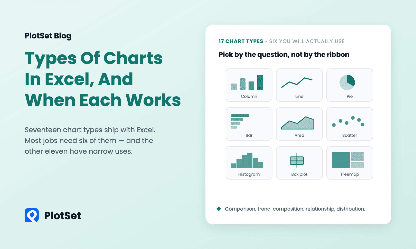
Orientation is the only difference. Use horizontal bars when your category names are long: "Marketing and Communications" gets a full line to itself instead of being rotated 45 degrees or truncated to "Marketing and...". Use vertical columns, covered in the column chart guide, for short labels or a handful of time periods.
The three fixes that matter
Excel's defaults are tuned for speed, not for reading. These three take about a minute between them and account for most of the difference between a default chart and a good one.
1. Sort the bars
An unsorted bar chart makes the reader do the ranking themselves. Unless your categories have their own natural order (months, age bands, survey answers from "strongly agree" to "strongly disagree"), sort them by value.
Do it in the data, not the chart: select your range, then Data → Sort, and sort by the value column. The chart follows.
One quirk to know about: Excel plots horizontal bar charts bottom-up, so a descending sort in the sheet produces an ascending chart. Either sort ascending in the sheet, or right-click the category axis → Format Axis → tick Categories in reverse order.
2. Use one colour
Excel gives multi-series charts a different colour per series, which is right. For a single series it sometimes still varies the fill, which is not: with one series, colour encodes nothing, and a rainbow of bars just adds visual noise.
Click any bar once to select the whole series, then use Format → Shape Fill to set one colour for all of them. If you want to draw attention to a particular bar, click it a second time to select only that bar and give it an accent colour. One highlighted bar in a field of grey is far more effective than eight competing colours. Our guide to using colour in data visualization explains why.
3. Add value labels, drop the gridlines
Click the chart, hit the + button in the top right, and tick Data Labels. Now the numbers are printed at the end of each bar and nobody has to measure against the axis.
Once the labels are there, the gridlines are redundant: untick Gridlines in the same menu. You can usually drop the value axis too.
Things that will trip you up
The axis does not start at zero. Bar length is the encoding, so a truncated axis exaggerates every difference on the chart. Excel normally starts at zero on its own, but it will not if you have negative values or if you changed the minimum earlier. Right-click the value axis → Format Axis → set Minimum to 0.
Excel charted the wrong direction. If your categories ended up on the value axis, click the chart and use Chart Design → Switch Row/Column.
Adding new rows does not update the chart. A plain range is fixed at the size it was when you inserted the chart. Convert the range to a table first (select it, Ctrl + T), and any row you add is included automatically.
The chart is too dense. Twenty-five bars is about the practical ceiling, especially horizontally. Beyond that, filter to a meaningful top group, or show the distribution instead of every individual category. To compare several series per category, a grouped bar chart or a stacked bar chart is the next step up.
When Excel is the wrong tool
Excel is good at exploring your own data. It becomes awkward the moment the chart has to leave the spreadsheet: pasting it into a document usually flattens it to an image, putting it on a web page means exporting a picture or using an Office embed, and matching a brand's fonts and colours means restyling it by hand every time.
Here is the same two-column layout, sorted, in one colour and with value labels, published as a live PlotSet chart. The data is the 2023 GDP of six EU economies from the World Bank, rounded to US$ billions.
If the chart is going onto a website, into a report that has to match a brand, or in front of an audience who might want to hover over a bar, it is worth building it somewhere designed for publishing. The PlotSet bar chart maker takes the same two columns (save a CSV from Excel and upload it, or paste them straight in) and gives you an interactive chart with your own fonts and colours, a live embed snippet, and PNG, SVG and JPG export. It is free to start, and the bar chart guide walks through it step by step. Charting a relationship between two numbers instead? See how to make an XY scatter graph in Excel.
Quick reference
| Task | How |
|---|---|
| Insert default chart | Select data, Alt + F1 |
| Insert on its own sheet | Select data, F11 |
| Preview chart options | Ctrl + Q |
| Swap axes | Chart Design → Switch Row/Column |
| Sort the bars | Sort the source data, then reverse the category axis |
| Add value labels | Chart + button → Data Labels |
| Force a zero baseline | Right-click value axis → Format Axis → Minimum 0 |
Frequently asked questions
How do I make a bar chart in Excel with two columns?
Select both columns including the header row, go to Insert → Charts, and pick Clustered Bar. The first column becomes the category labels and the second becomes the bar lengths.
What is the difference between a bar chart and a column chart in Excel?
Orientation only. Bar charts run horizontally and suit long category names; column charts run vertically and suit short labels or time periods.
How do I sort a bar chart from largest to smallest in Excel?
Sort the source data by the value column with Data → Sort. Because Excel draws horizontal bars from the bottom up, also tick Categories in reverse order on the category axis, or sort the sheet ascending.
How do I add numbers to the bars?
Click the chart, press the + button in its top right corner and tick Data Labels. The value then prints at the end of each bar, and you can remove the gridlines.
How do I make a bar chart in Excel that I can embed on a website?
Once a chart leaves the workbook it is usually a static picture. To get an interactive chart you can embed, save the two columns as a CSV and upload them to a chart tool such as the PlotSet bar chart maker.